Homework 03 Solutions

Getting Ready

• Load in the dataset “zombies.csv” from my GitHub repo.

The first element of this assignment is loading in the dataset. As always in R, there are many many ways to do this, and we have examples for a few of them in previous modules (particularly Module 05). My preferred way, when I’ve got a clear online location for the dataset (in this case, the GitHub repo link provided above), is to use a {curl} command just because that’s usually the most efficient. As always, though, if you have another way to do it that’s great; the point is to get the data in, doesn’t necessarily matter how for a dataset this small:

> library(curl)
> f <- curl("https://raw.githubusercontent.com/fuzzyatelin/fuzzyatelin.github.io/master/AN588_Fall23/zombies.csv")
> z <- read.csv(f, header = TRUE, sep = ",", stringsAsFactors = FALSE)
> head(z)

##   id first_name last_name gender   height   weight zombies_killed
## 1  1      Sarah    Little Female 62.88951 132.0872              2
## 2  2       Mark    Duncan   Male 67.80277 146.3753              5
## 3  3    Brandon     Perez   Male 72.12908 152.9370              1
## 4  4      Roger   Coleman   Male 66.78484 129.7418              5
## 5  5      Tammy    Powell Female 64.71832 132.4265              4
## 6  6    Anthony     Green   Male 71.24326 152.5246              1
##   years_of_education                           major      age
## 1                  1                medicine/nursing 17.64275
## 2                  3 criminal justice administration 22.58951
## 3                  1                       education 21.91276
## 4                  6                  energy studies 18.19058
## 5                  3                       logistics 21.10399
## 6                  4                  energy studies 21.48355

Great! Now we can get started characterizing this population of zombie apocalypse survivors, including taking the population mean and standard deviation for each quantitative random variable.

Question 1

• Calculate the population mean and standard deviation for each quantitative random variable (height, weight, age, number of zombies killed, and years of education).

Remember, this is different from sample statistics, as outlined in Module 08, where you can find helpful code for calculating them. In that module, we learned that while the population variance is the sum of squares divided by N (our population size), the sample variance is the sum of squares divided by n-1 (our sample size minus one degree of freedom).

We can use the mean() function to calculate the mean of, for example, weight:

> mean(z$weight)

## [1] 143.9075

And let’s use the pop_sd function we created in Module 08 to get the population standard deviation (we also need the pop_v function to make it work properly):

> pop_v <- function(x) {
+     sum((x - mean(x))^2)/(length(x))
+ }
> pop_sd <- function(x) {
+     sqrt(pop_v(x))
+ }
> pop_sd(z$weight)

## [1] 18.39186

If you compare it to the sd() function, designed for samples, you’ll see it’s slightly different due to the accommodation for the degrees of freedom:

> sd(z$weight)

## [1] 18.40106

Now, you can just run each of these one by one, simply plugging in the different variables, but the {tidyverse} has given us some fancier (and faster) options. You can use the summarise() function (or verb as the {tidyverse} calls them) to run all of them in a single pipe:

> library(tidyverse)
> zparams <- z %>%
+     select(height, weight, age, zombies_killed, years_of_education) %>%
+     summarise(across(everything(), list(mean = mean, sd = pop_sd)))
> zparams

##   height_mean height_sd weight_mean weight_sd age_mean   age_sd
## 1     67.6301   4.30797    143.9075  18.39186 20.04696 2.963583
##   zombies_killed_mean zombies_killed_sd years_of_education_mean
## 1               2.992          1.747551                   2.996
##   years_of_education_sd
## 1              1.675704

Alternatively (and, I think, much more elegantly), Natalia Kelley came up with this solution, which gives a much nicer and more readable output:

> s <- z %>%
+     select(height, weight, age, zombies_killed, years_of_education)
> 
> cbind(mean = apply(s, 2, mean), sd = apply(s, 2, pop_sd))

##                         mean        sd
## height              67.63010  4.307970
## weight             143.90748 18.391857
## age                 20.04696  2.963583
## zombies_killed       2.99200  1.747551
## years_of_education   2.99600  1.675704

Question 2

• Use {ggplot} to make boxplots of each of these variables by gender.

The easiest way to learn how to use {ggplot2} is to just dive in and start experimenting. You can get started by checking out the {tidyverse} webpage for {ggplot2}. There’s a really helpful cheat sheet there that will walk you through basic {ggplot2} grammar.

For a shortcut to drawing these plots, we can also go back and copy code used in Module 06

Now, to build a boxplot, we first need to use the ggplot function, which will set up our dataset, followed by a geom call that defines the kind of figure we want to make from that dataset. Here’s a first try making a boxplot if height by gender. It’s a very basic plot in which I’m calling in my dataset (data = z), defining my x- and y-axis variables (there are named in the aes() or aesthetics command within ggplot()), and then defining my figure output as a boxplot using the geom_boxplot() command. Notice that separate commands that modify the figure outside our ggplot() command are added using the + character:

> p <- ggplot(data = z, aes(x = gender, y = height))
> 
> p <- p + geom_boxplot()
> 
> p

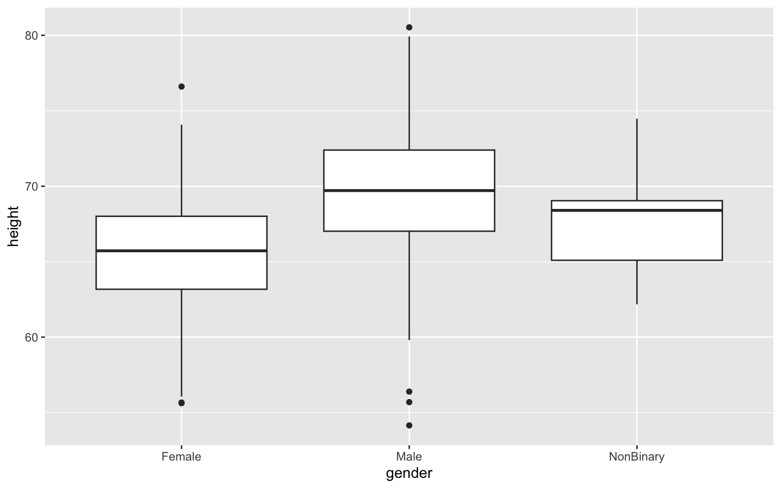
The really nice thing about {ggplot2} is the added capabilities to prettify your work. Here’s a small example… see if you can figure out which bit of code makes which change to the graphic (also, notice how I’ve broken up my code to make it clearly readable each time I modify the figure; this kind of syntax might be helpful to use while you’re learning {ggplot2}):

> p <- ggplot(data = z, aes(x = gender, y = height))
> 
> p <- p + geom_boxplot(aes(fill = gender))
> 
> p <- p + ggtitle("Height by Gender in Survivors")
> 
> p <- p + theme_bw()
> 
> p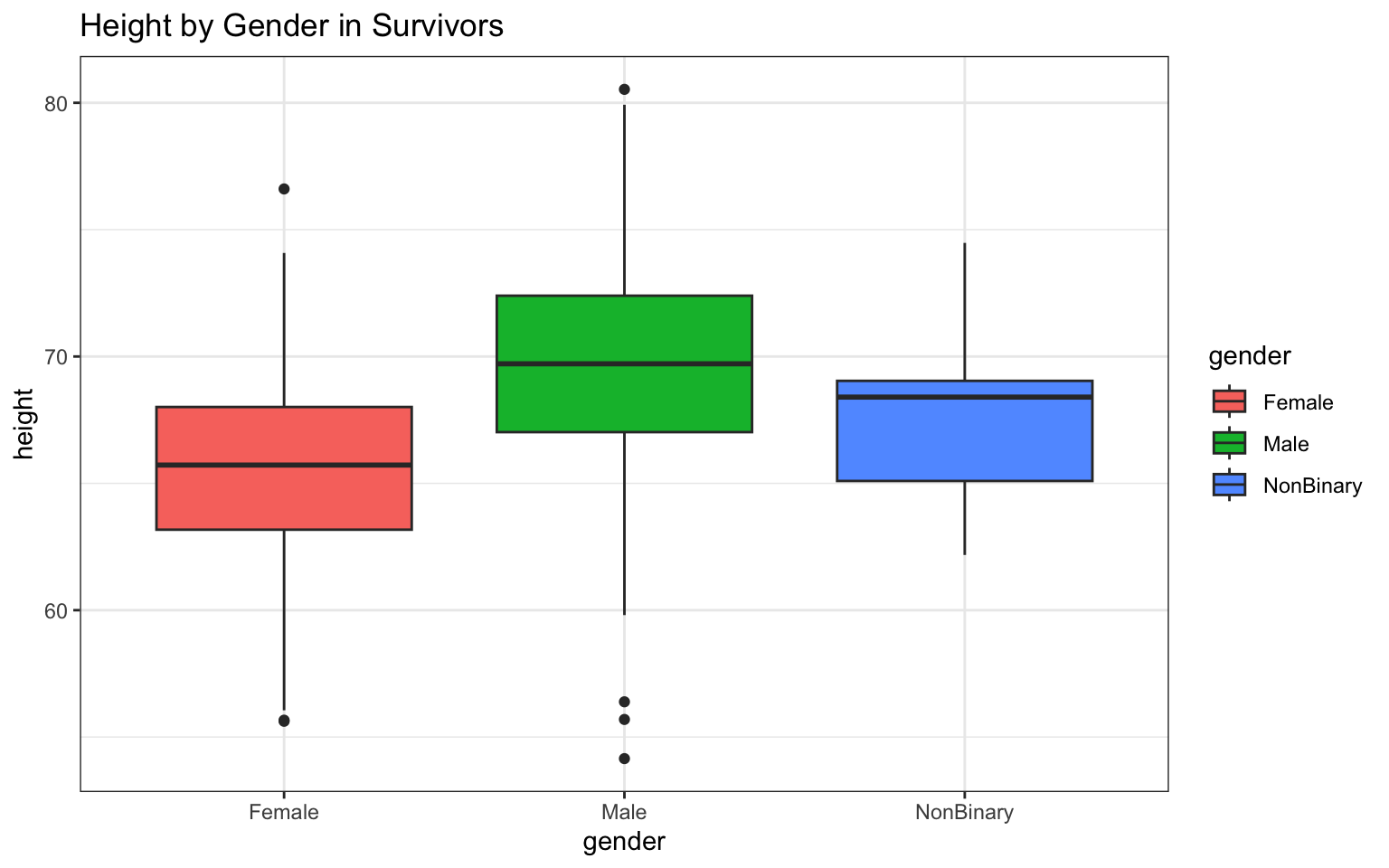

You can easily run all of the required plots by copying and pasting each individual variable name into the chunk, like so (notice I’ve used a more compact syntax here… one line of code per plot; convenient, but also maybe confusing):

> p <- ggplot(data = z, aes(x = gender, y = height)) + geom_boxplot(aes(fill = gender)) +
+     ggtitle("Height by Gender in Survivors") + theme_bw()
> p

> p <- ggplot(data = z, aes(x = gender, y = weight)) + geom_boxplot(aes(fill = gender)) +
+     ggtitle("Weight by Gender in Survivors") + theme_bw()
> p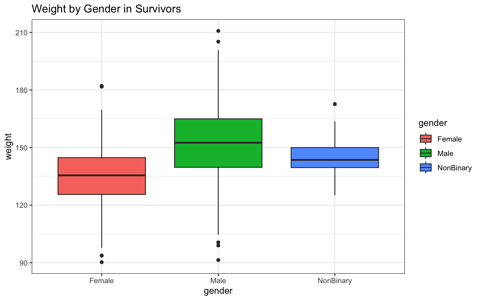

> p <- ggplot(data = z, aes(x = gender, y = zombies_killed)) + geom_boxplot(aes(fill = gender)) +
+     ggtitle("Zombies Killed by Gender in Survivors") + theme_bw()
> p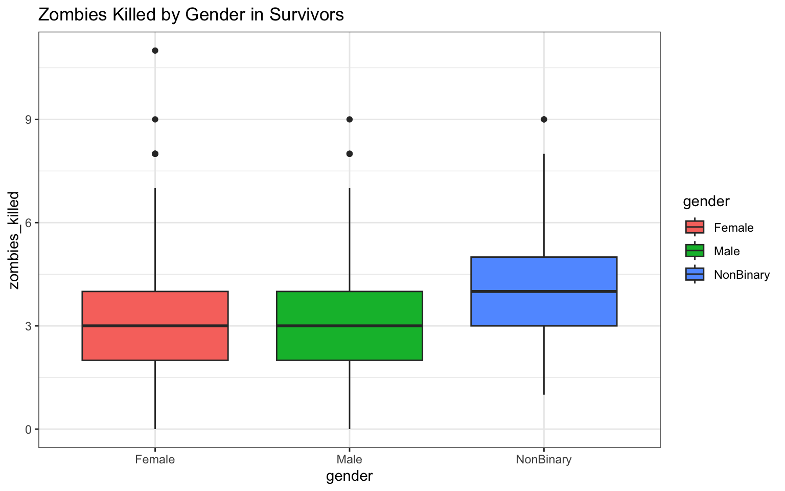

> p <- ggplot(data = z, aes(x = gender, y = years_of_education)) + geom_boxplot(aes(fill = gender)) +
+     ggtitle("Years of Education by Gender in Survivors") + theme_bw()
> p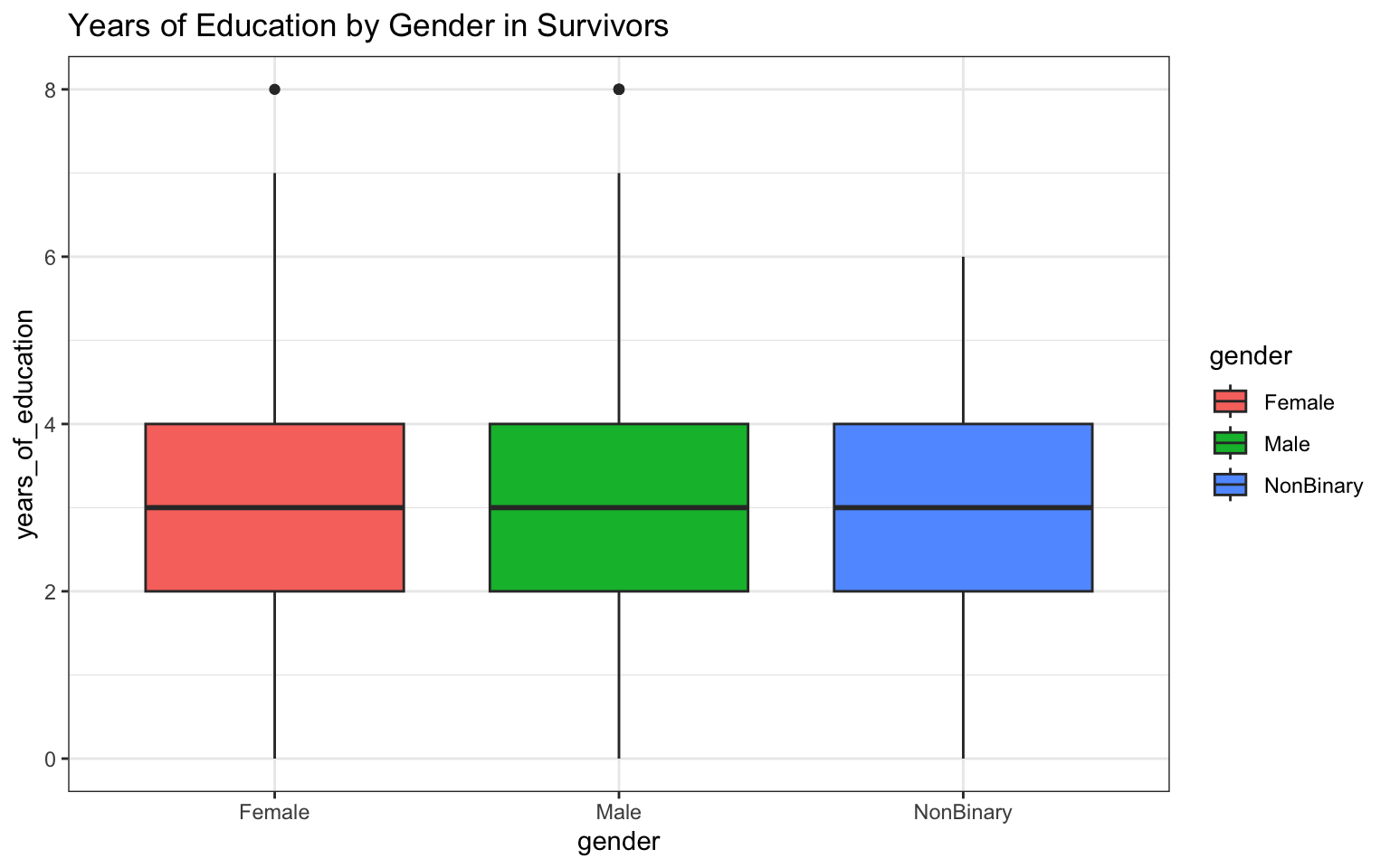

> p <- ggplot(data = z, aes(x = gender, y = age)) + geom_boxplot(aes(fill = gender)) +
+     ggtitle("Age by Gender in Survivors") + theme_bw()
> p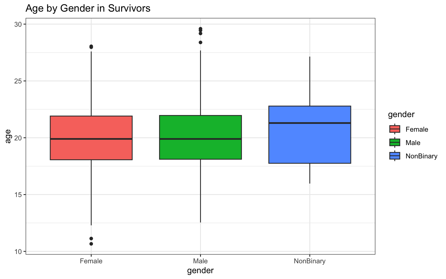

Now, as with the previous example, there are ways to simplify our work so that we don’t have to write a separate line of code for each figure. Remembering the value of looping to save time, I leaned on the package {ggloop} to run all my plots at once. I would not expect you to be able to figure this out on your own, but I thought it might be nice to show you (may come in handy later!):

> library(ggloop)
> # Here I use piping to select the names of only those columns in 'z' that
> # have numeric entries (plus the 'gender' column)
> traits <- z %>%
+     select(gender, height, weight, zombies_killed, years_of_education, age)
> 
> # Below is the code for using the {ggloop} package to make all the plots
> # at once. Can you see how the syntax for this package differs from
> # regular {ggplot2}?
> genplots <- ggloop(traits, aes_loop(x = gender, y = height:age))
> genplots[1:5] <- genplots[1:5] %L+% geom_boxplot(aes(fill = gender)) %L+% theme_bw()
> genplots

## $x.gender_y.height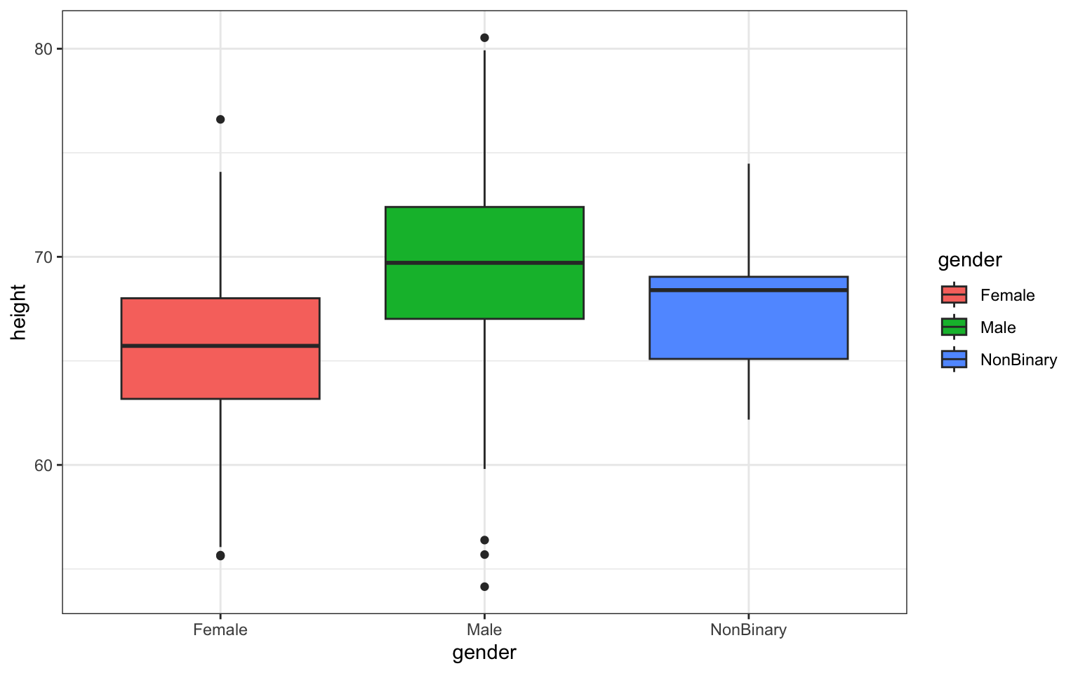

## 
## $x.gender_y.weight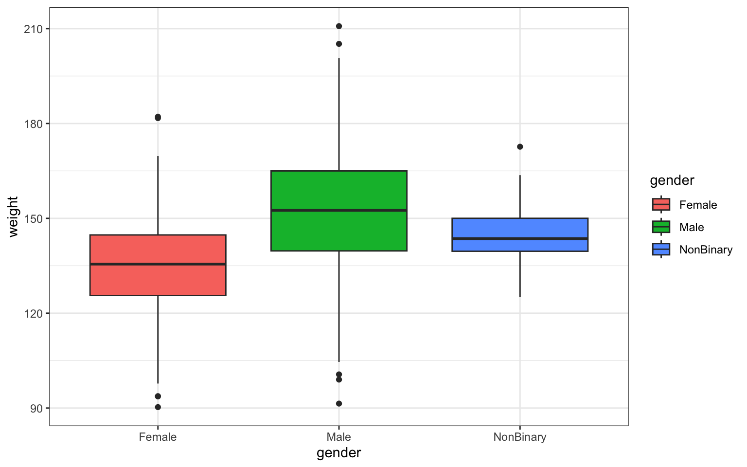

## 
## $x.gender_y.zombies_killed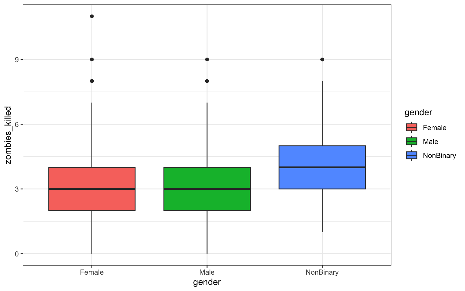

## 
## $x.gender_y.years_of_education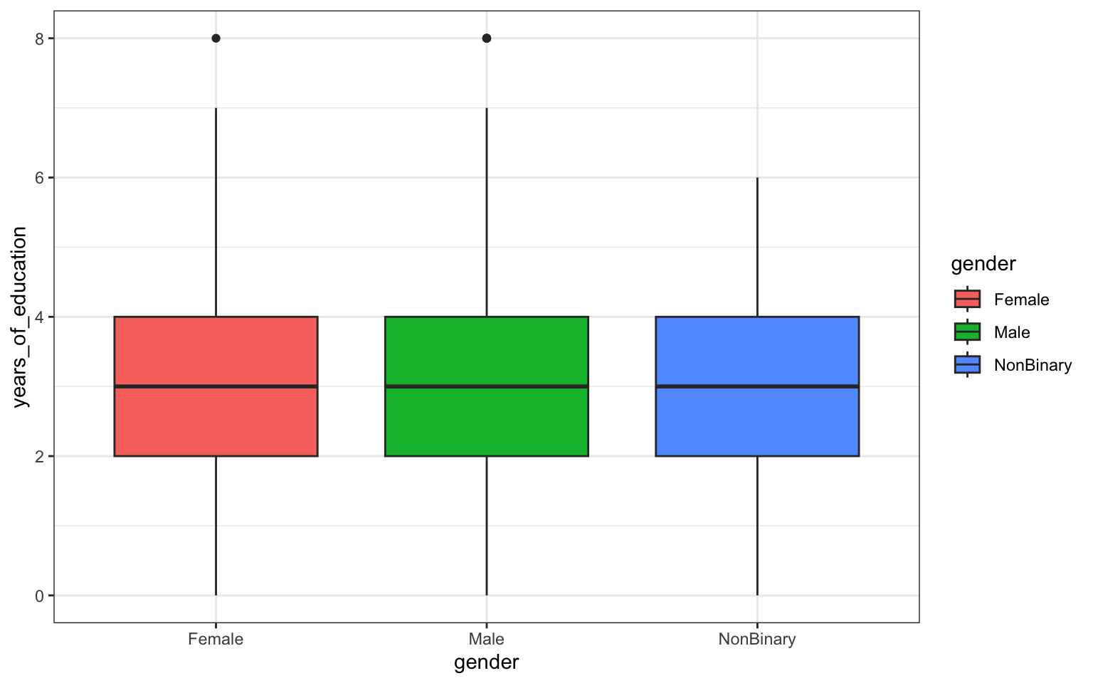

## 
## $x.gender_y.age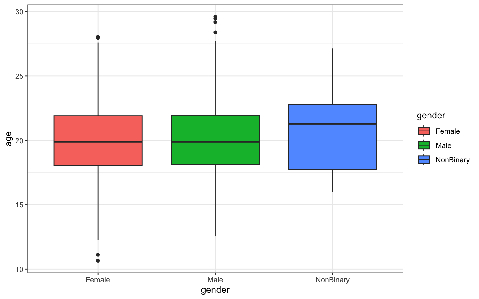

## 
## attr(,"class")
## [1] "gglist"

Question 3

• Use {ggplot} to make scatterplots of height and weight in relation to age. Do these variables seem to be related? In what way?

The easiest way to make a scatterplot from these data, given that we’ve already made a boxplot, is to simply copy and paste our boxplot code and 1) swap out our variables, and 2) change our geom_boxplot for the geom for a scatterplot, like geom_point, and finally 3) we should also rename the object we save the plot to, so we can keep versions of both plots in our R space:

> haplot <- ggplot(data = z, aes(x = age, y = height))
> 
> haplot <- haplot + geom_point()
> 
> haplot <- haplot + ggtitle("Height by Age in Survivors")
> 
> haplot <- haplot + theme_bw()
> 
> haplot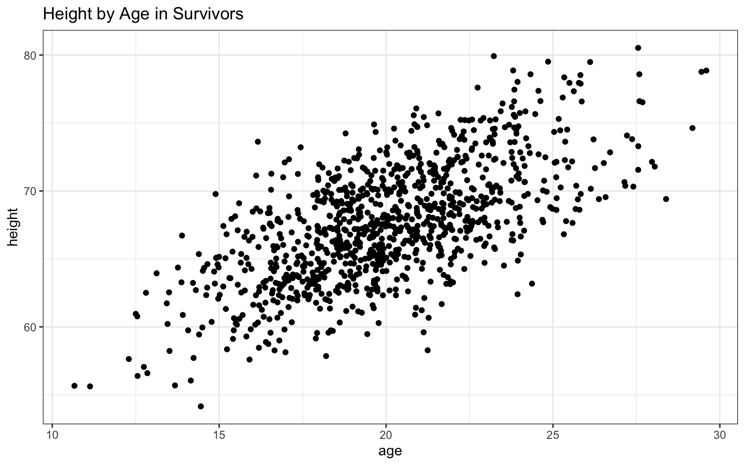

> waplot <- ggplot(data = z, aes(x = age, y = weight))
> 
> waplot <- waplot + geom_point()
> 
> waplot <- waplot + ggtitle("Weight by Age in Survivors")
> 
> waplot <- waplot + theme_bw()
> 
> waplot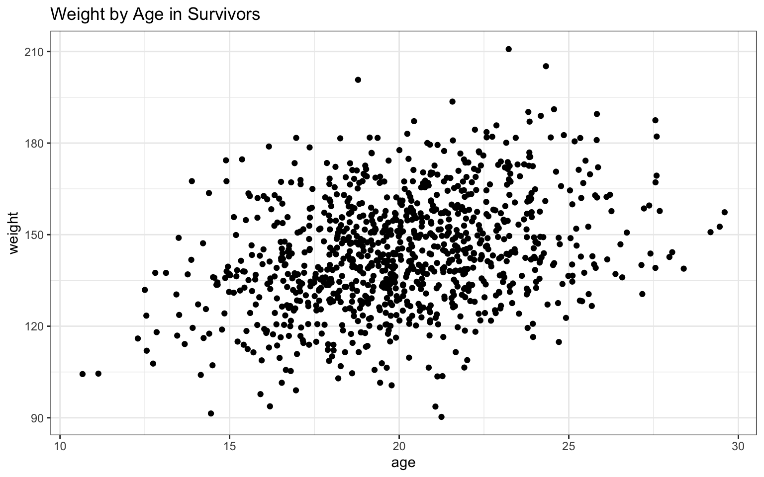

Based on the plots in Module 06, we can also add a trendline that really clearly illustrates the relationship between the two variables:

> haplot <- haplot + geom_smooth(method = "lm")
> 
> haplot

## `geom_smooth()` using formula = 'y ~ x'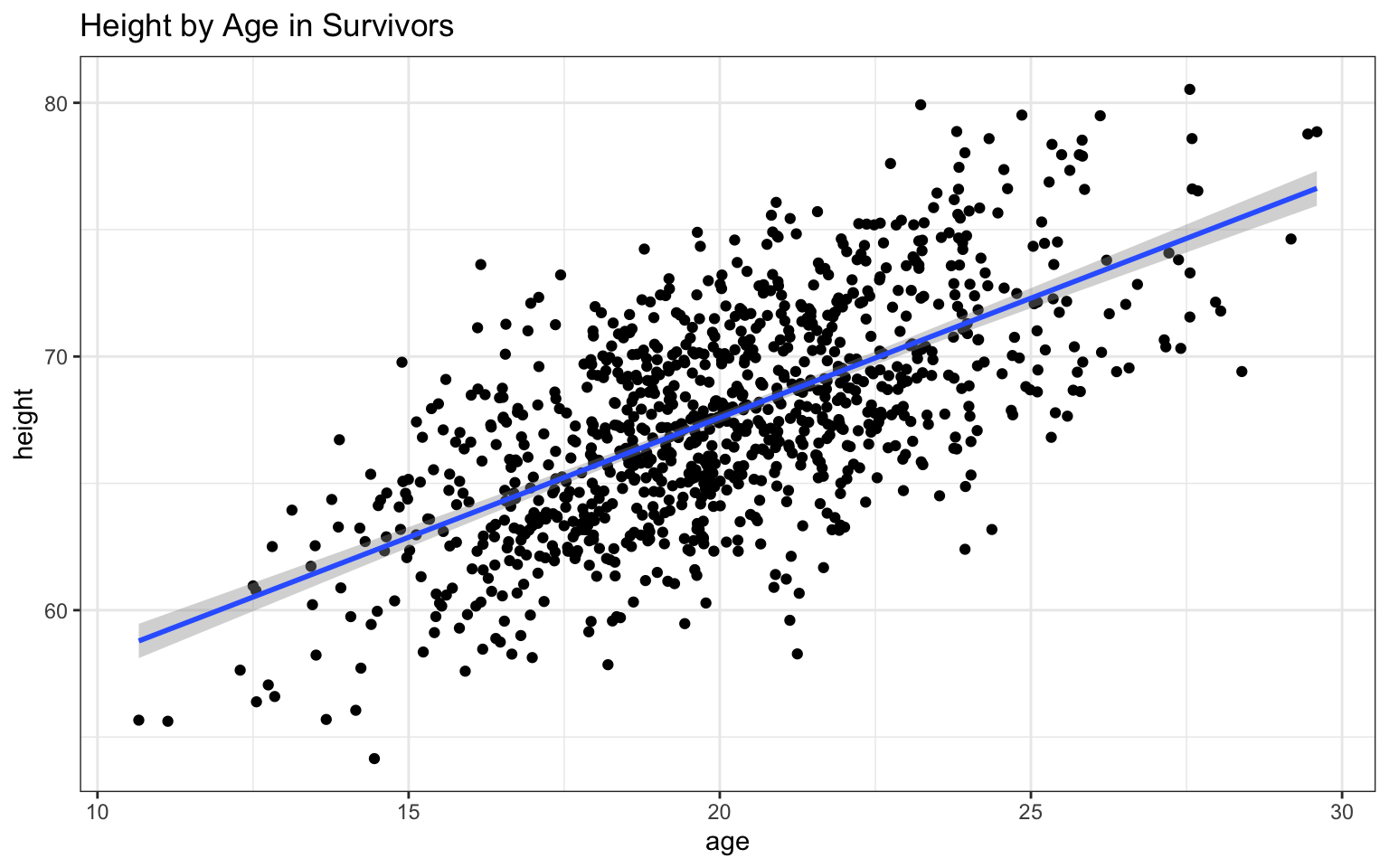

> waplot <- waplot + geom_smooth(method = "lm")
> 
> waplot

## `geom_smooth()` using formula = 'y ~ x'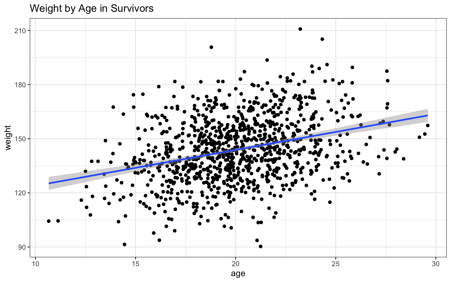

In this case, both variables appear to be positively related to age, with both height and, to a lesser extent, weight increasing as age increases. The addition of the regression lines really highlights these relationships, no?

Question 4

• Using histograms and Q-Q plots, check whether the quantitative variables seem to be drawn from a normal distribution. Which seem to be and which do not (hint: not all are drawn from the normal distribution)? For those that are not normal, can you determine from which common distribution they are drawn?

Let’s go back to base R plotting to look at these all together using the par() command:

> par(mfrow = c(2, 3))  # gives us three panels in two rows
> attach(z)
> hist(height, freq = FALSE, main = "height", xlab = "height", ylab = "density",
+     ylim = c(0, 0.3))
> hist(weight, freq = FALSE, main = "weight", xlab = "weight", ylab = "density",
+     ylim = c(0, 0.3))
> hist(age, freq = FALSE, main = "age", xlab = "age", ylab = "density", ylim = c(0,
+     0.3))
> hist(zombies_killed, freq = FALSE, main = "zombies killed", xlab = "zombies killed",
+     ylab = "density", ylim = c(0, 0.3))
> hist(years_of_education, freq = FALSE, main = "years of education", xlab = "years of education",
+     ylab = "density", ylim = c(0, 0.3))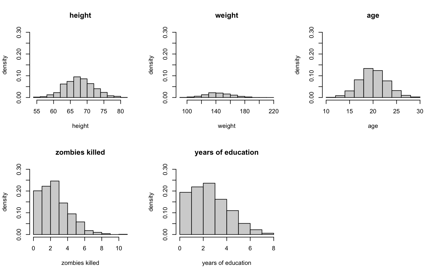

Just eye-balling it, I’d say that height and age look normal, and maybe weight (which looks a bit skewed), but zombies killed and years of education both look very non-normal (given that we would be counting the number of zombies killed and the number of years of school, I’d guess they’re probably Poisson-ish).

Let’s look at the QQ plots. We’ll use the method from earlier in Module 08:

> par(mfrow = c(2, 3))  # gives us three panels in two rows
> 
> qqnorm(z$height, main = "Normal QQ plot height")
> qqline(z$height, col = "gray")
> 
> qqnorm(z$weight, main = "Normal QQ plot weight")
> qqline(z$weight, col = "gray")
> 
> qqnorm(z$age, main = "Normal QQ plot age")
> qqline(z$age, col = "gray")
> 
> qqnorm(z$zombies_killed, main = "Normal QQ plot zombies killed")
> qqline(z$zombies_killed, col = "gray")
> 
> qqnorm(z$years_of_education, main = "Normal QQ plot education")
> qqline(z$years_of_education, col = "gray")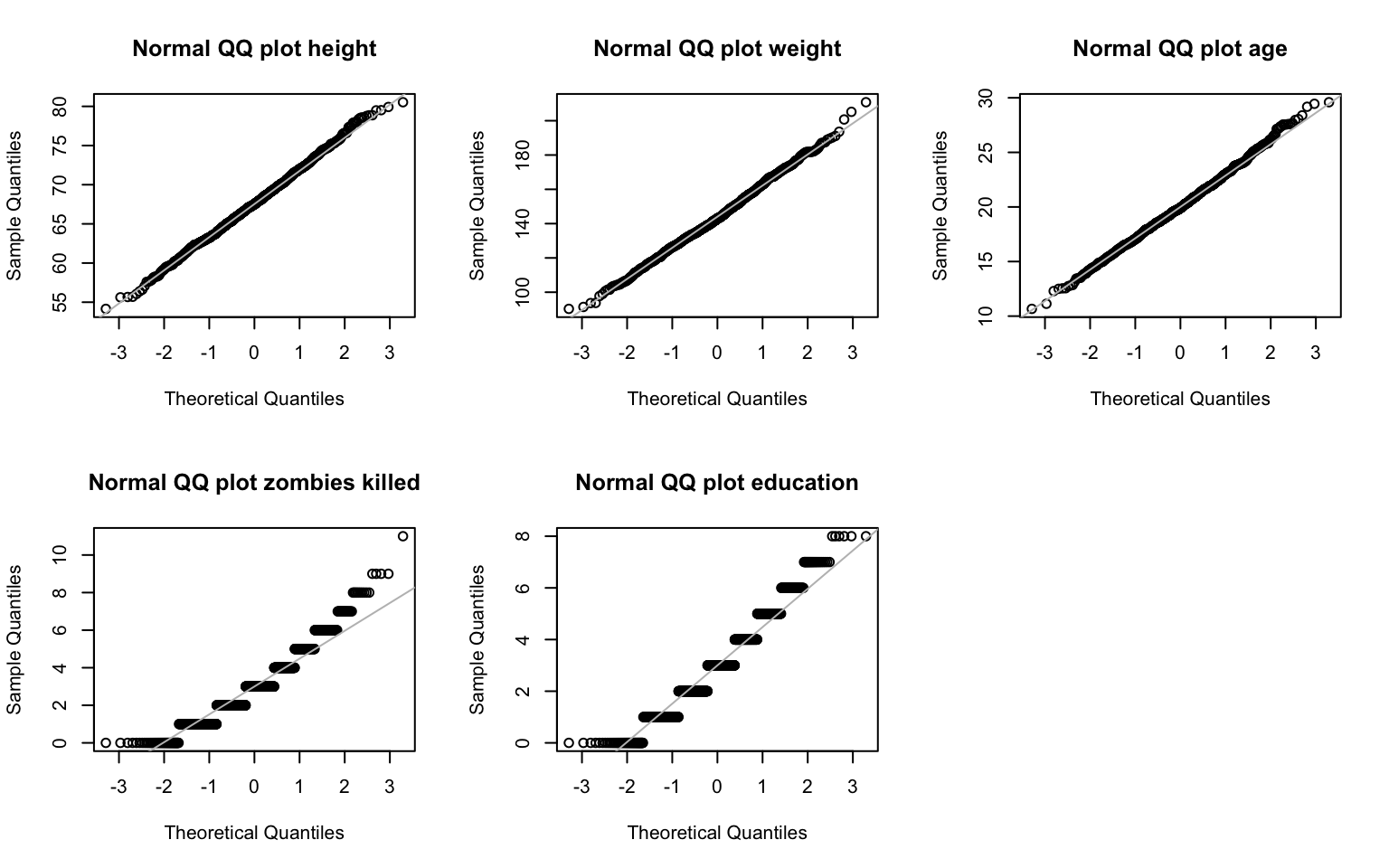

Well, weight looks ok, but sure enough it looks like zombies killed and years of education don’t easily fit a normal distribution!

Now, to assess whether these two are more Poisson-ish, we can do what we did in Homework-02 and compare these distributions to the hypothetical Poisson distribution of the data and see if they match.

Let’s experiment with zombies_killed… our x should be no greater than the maximum number of kills (in this case, 11), and our lambda would be roughly the average probability of a kill (or the mean). Let’s also use par() again to make this visually easier (and with thanks to Diego Alonso Larre for the simple code for making the second figure):

> par(mfrow = c(1, 2))  # gives us two panels in one row
> 
> hist(zombies_killed, freq = FALSE, main = "zombies killed", xlab = "zombies killed",
+     ylab = "density", ylim = c(0, 0.3), xlim = c(0, 11))
> 
> hist(rpois(1000, 3), probability = T)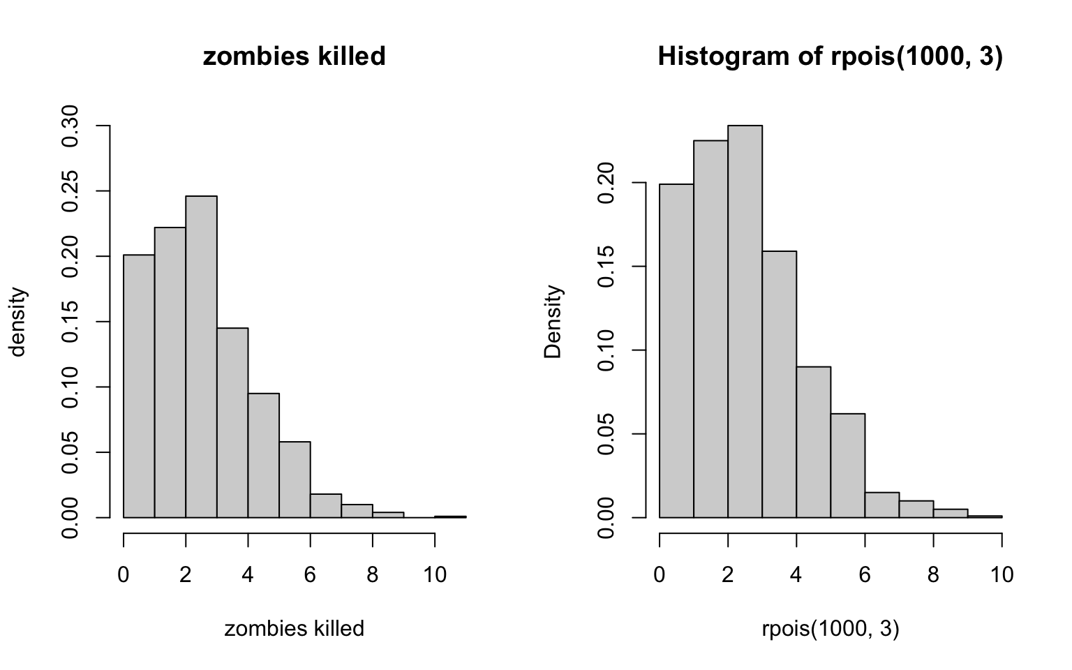

Hmmm… that doesn’t quite look right, does it? Let’s try another distribution. Maybe the Bernoulli?

To assess whether this is more Bernoulli-ish, we can do what we did in Homework-02 and compare these distributions to the hypothetical Bernoulli distribution of the data and see if they match. Let’s experiment… our x should be no greater than the maximum number of kills (in this case, 11), size is 1000 (that’s how many outcomes we’ve got), and from there we can experiment with the probability of a kill. As before, we’ll use par() again to make this visually easier:

> par(mfrow = c(1, 2))  # gives us two panels in one row
> 
> hist(zombies_killed, freq = FALSE, main = "zombies killed", xlab = "zombies killed",
+     ylab = "density", ylim = c(0, 0.3), xlim = c(0, 11))
> 
> probset2 <- dbinom(x = 0:11, size = 1000, prob = 1/550)
> barplot(probset2, names.arg = 0:11, space = 0, xlab = "kills", ylab = "Pr(X=outcome)",
+     ylim = c(0, 0.3), xlim = c(0, 11))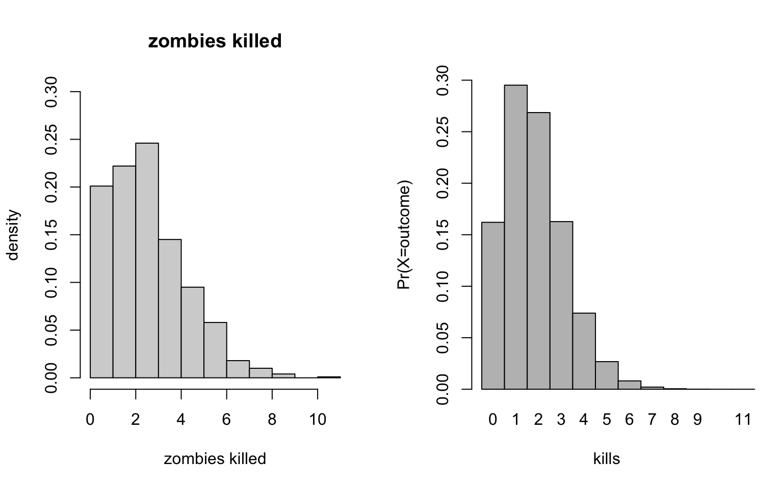

Ok… these look pretty similar to the data distributions, actually. Looks like the number of zombes killed come from our old friend the Bernoulli distribution.

Question 5

• Now use the sample() function to sample ONE subset of 30 zombie survivors (without replacement) from this population and calculate the mean and sample standard deviation for each variable. Also estimate the standard error for each variable and construct the 95% confidence interval for each mean. Note that for the variables that are not drawn from the normal distribution, you will need to base your estimate of the CIs on some different distribution.

Code for sample() we can get from Module 08, while code for confidence intervals we can get from Module 07. Don’t forget to define se(), which isn’t in the native R environment (you can either write your own function, as in the module, or load the sciplot package as a shortcut)!

> library(sciplot)
> 
> # For height:
> s_height <- sample(z$height, size = 30, replace = FALSE)
> mean(s_height)

## [1] 68.10931

> sd(s_height)

## [1] 3.976491

> upper_h <- mean(s_height) + qnorm(0.975, mean = 0, sd = 1) * se(s_height)
> lower_h <- mean(s_height) + qnorm(0.025, mean = 0, sd = 1) * se(s_height)
> ci_h <- c(lower_h, upper_h)
> ci_h

## [1] 66.68637 69.53225

> # For weight:
> s_weight <- sample(z$weight, size = 30, replace = FALSE)
> mean(s_weight)

## [1] 144.4021

> sd(s_weight)

## [1] 16.77679

> upper_w <- mean(s_weight) + qnorm(0.975, mean = 0, sd = 1) * se(s_weight)
> lower_w <- mean(s_weight) + qnorm(0.025, mean = 0, sd = 1) * se(s_weight)
> ci_w <- c(lower_w, upper_w)
> ci_w

## [1] 138.3987 150.4055

> # For age:
> s_age <- sample(z$age, size = 30, replace = FALSE)
> mean(s_age)

## [1] 19.60539

> sd(s_age)

## [1] 2.640367

> upper_a <- mean(s_age) + qnorm(0.975, mean = 0, sd = 1) * se(s_age)
> lower_a <- mean(s_age) + qnorm(0.025, mean = 0, sd = 1) * se(s_age)
> ci_a <- c(lower_a, upper_a)
> ci_a

## [1] 18.66057 20.55022

Now, for the non-normal samples, we can’t rely on the above code because it assumes normality and we already know these aren’t normally distributed! Here, we’ll have to use bootstrapping, as also done in Module 07:

> # For zombies_killed:
> s_zombies_killed <- sample(z$zombies_killed, size = 30, replace = FALSE)
> mean(s_zombies_killed)

## [1] 2.766667

> sd(s_zombies_killed)

## [1] 1.994533

> set <- NULL  # sets up a dummy variable to hold our simulations
> n <- 15
> for (i in 1:10000) {
+     set[i] <- mean(sample(s_zombies_killed, n, replace = TRUE))
+ }
> quantile(set, c(0.025, 0.975))

##  2.5% 97.5% 
##   1.8   3.8

> # For years_of_education:
> s_years_of_education <- sample(z$years_of_education, size = 30, replace = FALSE)
> mean(s_years_of_education)

## [1] 2.9

> sd(s_years_of_education)

## [1] 1.626293

> set <- NULL  # sets up a dummy variable to hold our simulations
> n <- 15
> for (i in 1:10000) {
+     set[i] <- mean(sample(s_years_of_education, n, replace = TRUE))
+ }
> quantile(set, c(0.025, 0.975))

##     2.5%    97.5% 
## 2.133333 3.733333

Question 6

• Now draw 99 more random samples of 30 zombie survivors out and calculate the mean for each of the these samples. Together with the first sample you drew out, you now have a set of 100 means for each variable (each based on 30 observations), which constitutes a sampling distribution for each variable. What are the means and standard deviations of this distribution for each variable? How do the standard deviations compare to the standard errors estimated in the last exercise? What do these sampling distributions look like? Are they normally distributed? What about for those variables that you concluded were not originally drawn from a normal distribution?

> x_m_height <- NULL
> for (i in 1:100) {
+     x_m_height[i] <- mean(sample(z$height, 30))
+ }
> 
> hist(x_m_height, probability = TRUE)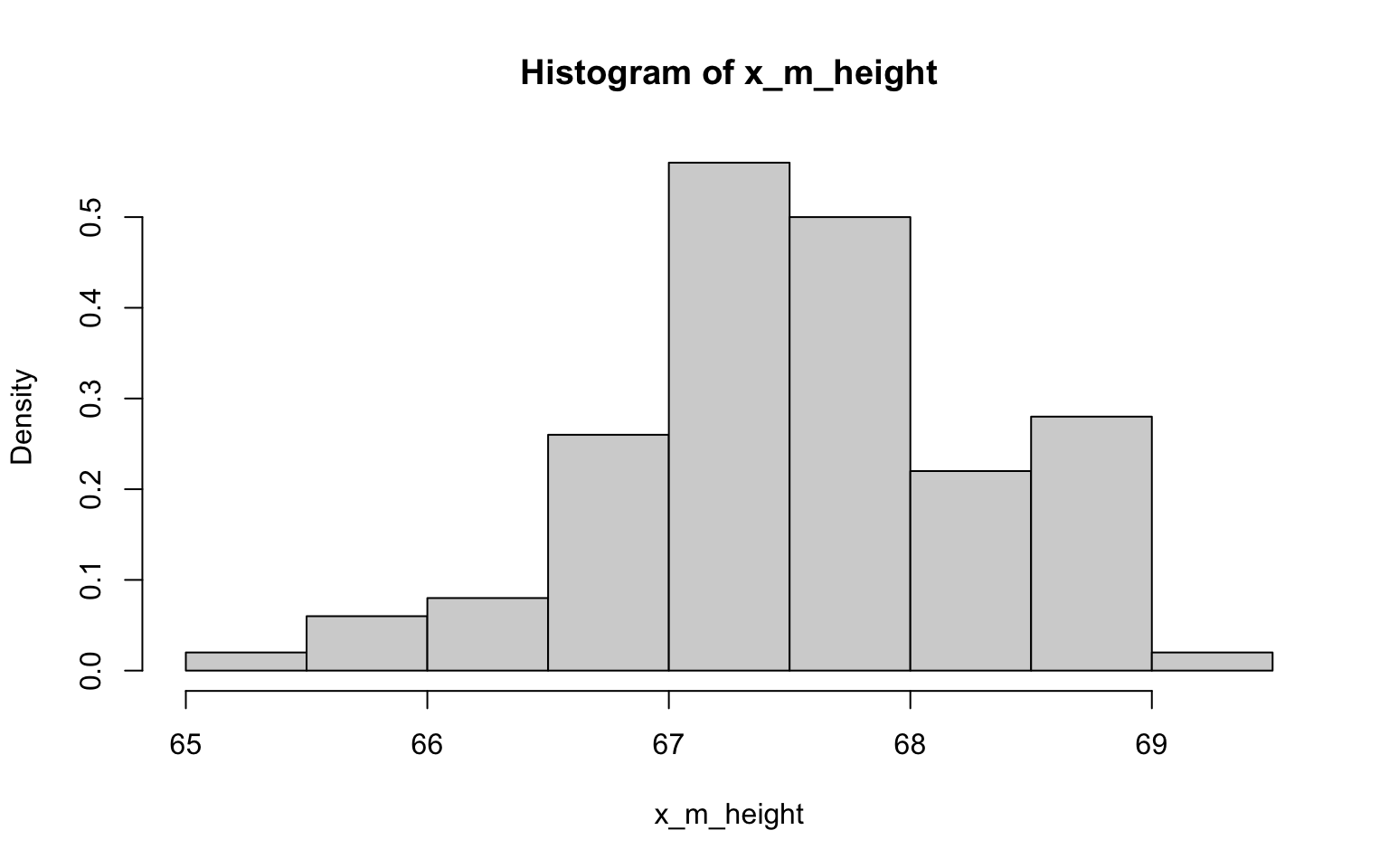

> mean(x_m_height)

## [1] 67.56361

> sd(x_m_height)

## [1] 0.7741392

> x_m_weight <- NULL
> for (i in 1:100) {
+     x_m_weight[i] <- mean(sample(z$weight, 30))
+ }
> 
> hist(x_m_weight, probability = TRUE)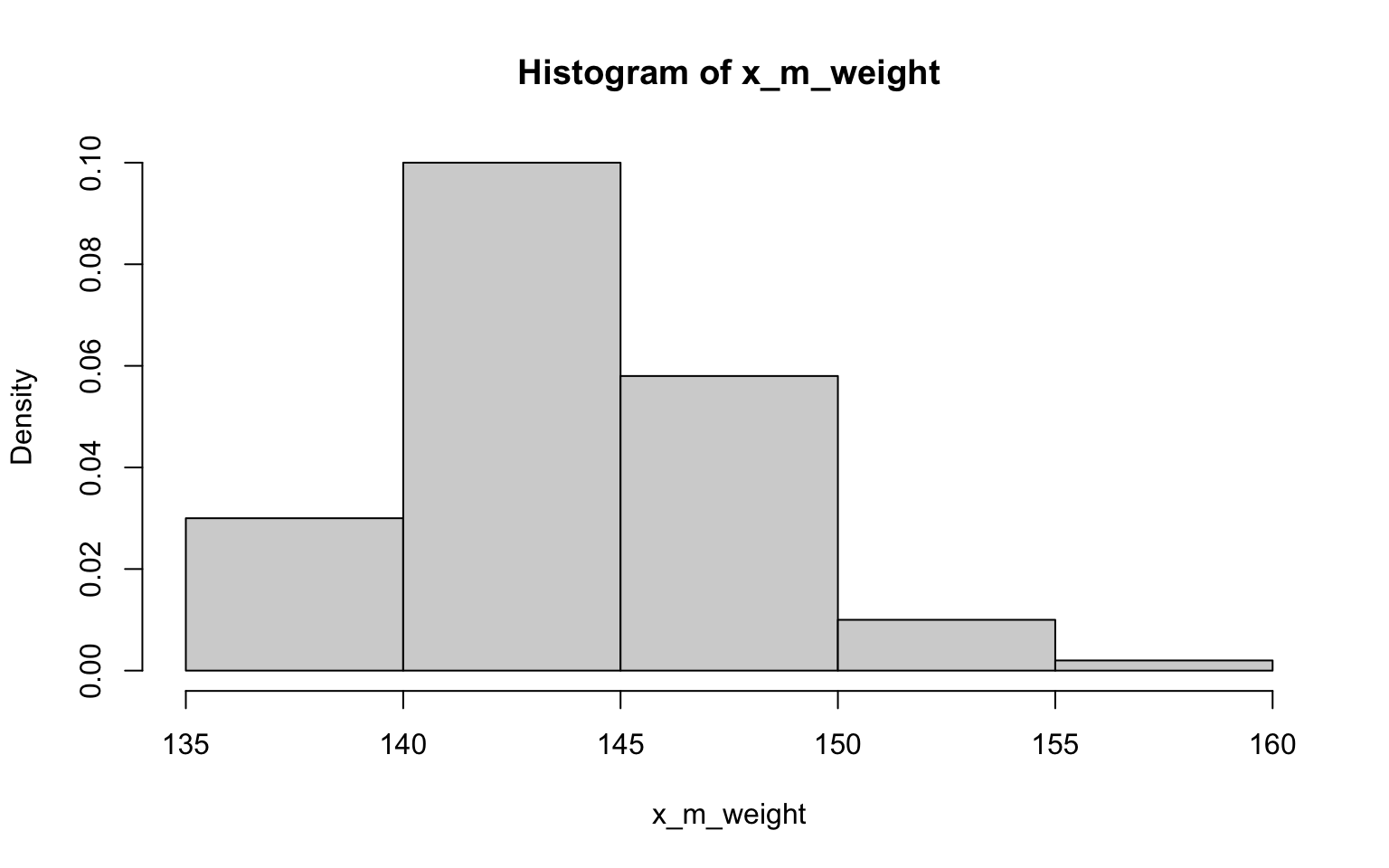

> mean(x_m_weight)

## [1] 143.769

> sd(x_m_weight)

## [1] 3.805587

> x_m_age <- NULL
> for (i in 1:100) {
+     x_m_age[i] <- mean(sample(z$age, 30))
+ }
> 
> hist(x_m_age, probability = TRUE)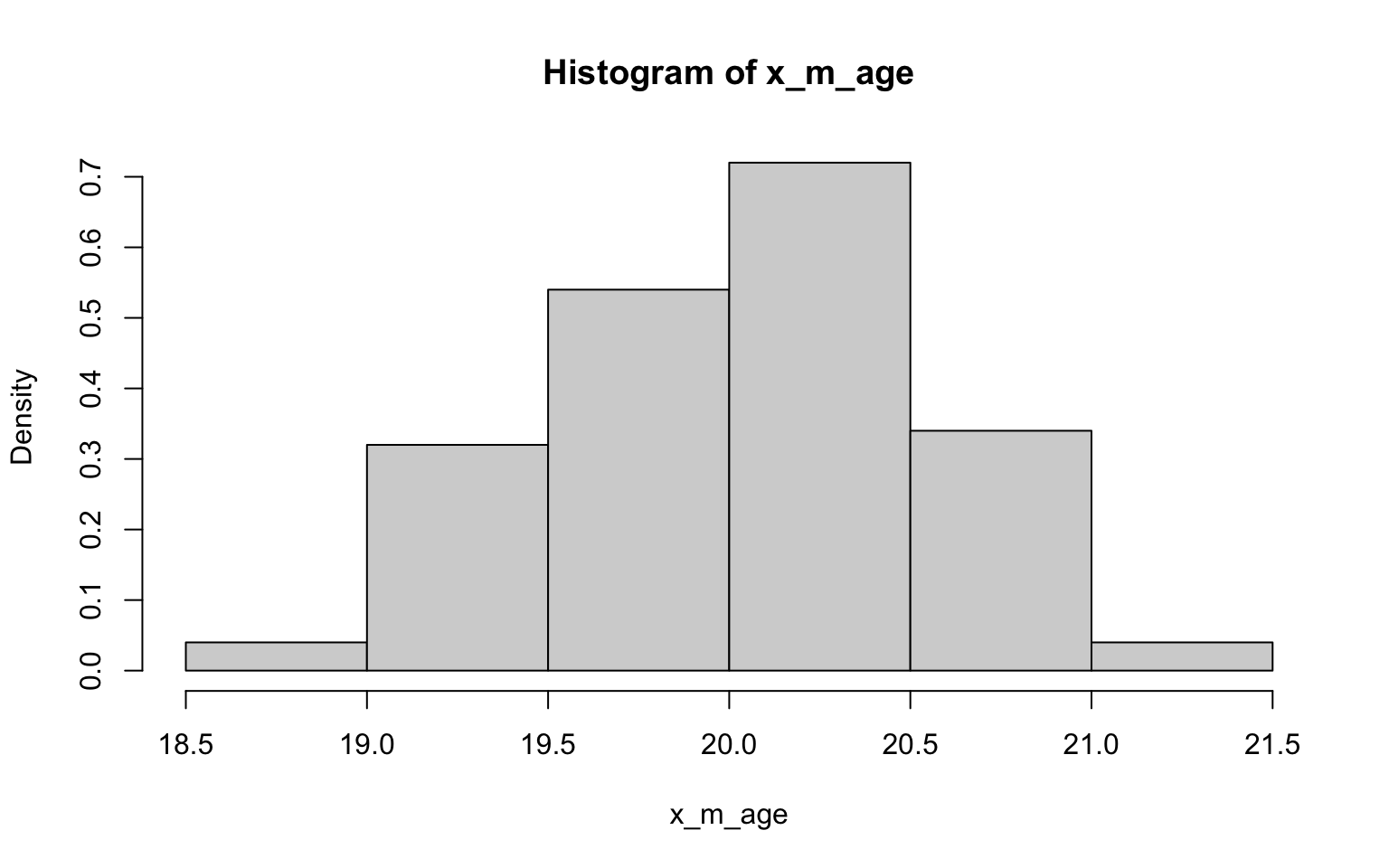

> mean(x_m_age)

## [1] 20.02224

> sd(x_m_age)

## [1] 0.5290551

> x_m_kill <- NULL
> for (i in 1:100) {
+     x_m_kill[i] <- mean(sample(z$zombies_killed, 30))
+ }
> 
> hist(x_m_kill, probability = TRUE)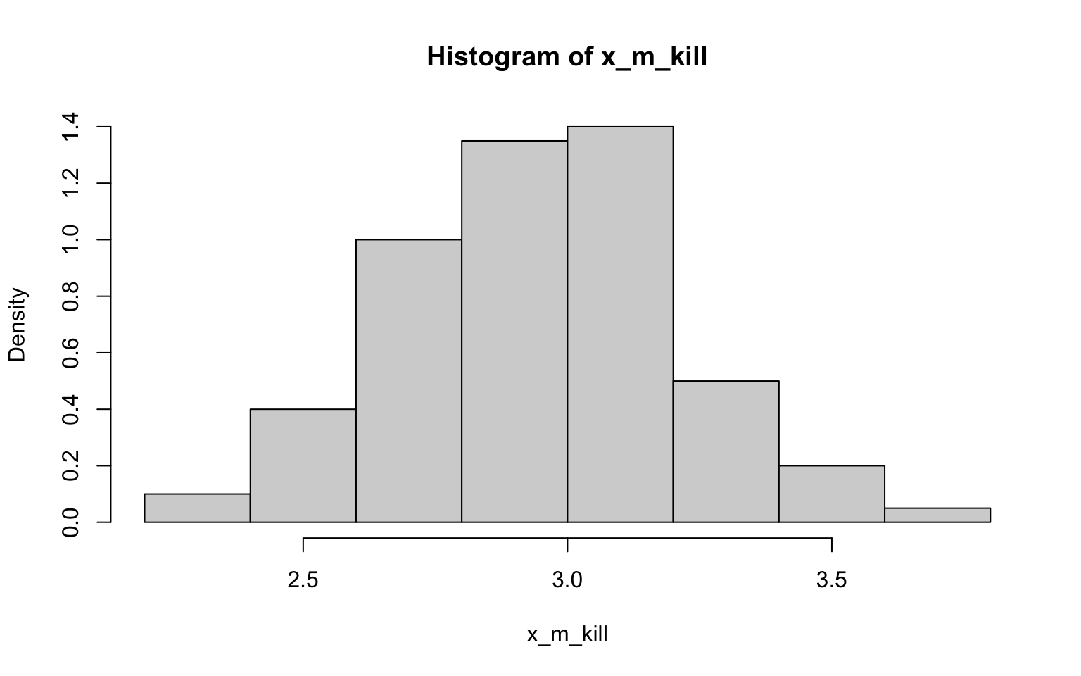

> mean(x_m_kill)

## [1] 2.965667

> sd(x_m_kill)

## [1] 0.2673583

> x_m_edu <- NULL
> for (i in 1:100) {
+     x_m_edu[i] <- mean(sample(z$years_of_education, 30))
+ }
> 
> hist(x_m_edu, probability = TRUE)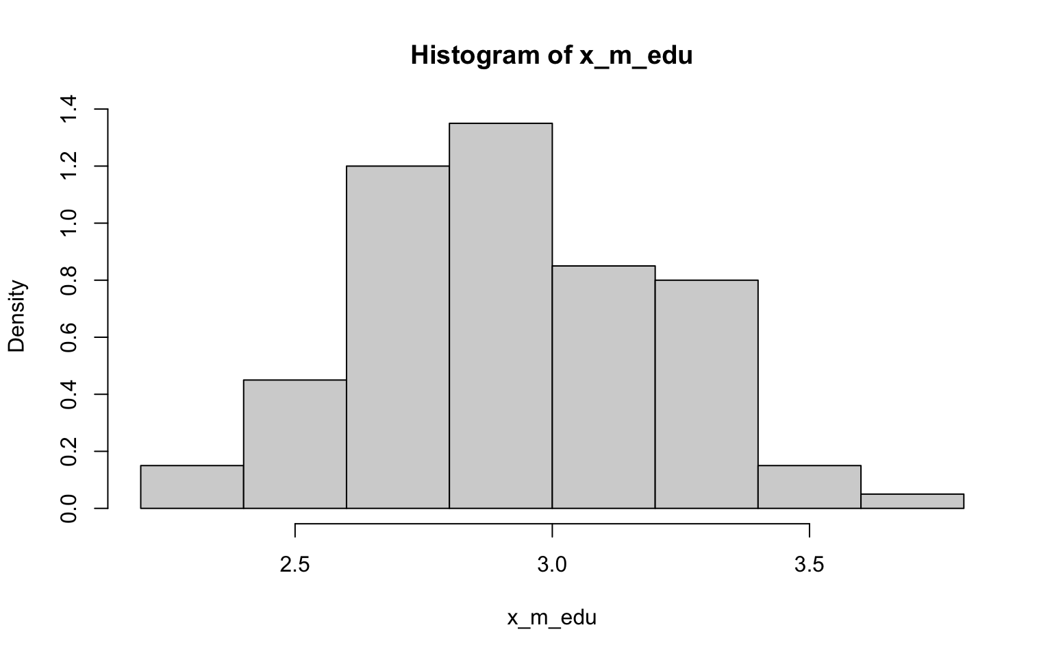

> mean(x_m_edu)

## [1] 2.924333

> sd(x_m_edu)

## [1] 0.2893491

Well, I have to say that the histograms here all look fairly normally distributed, including those derived from data with non-normal distributions (ok, so they may randomly look a bit wonkier than normal)… of course, that’s exactly what we’d expect in accordance with the CLT (yes, this was another way to illustrating the importance of this concept)! Also in accordance with the CLT, it looks like the SE’s estimated in the previous exercise the SDs are not quite the same, but are closer to each other than the SD of each as estimated in the previous exercise.